Corruption indicators in Mexico

As you can see there is only a slight positive correlation between the corruption index of the Mexican chapter of Transparency International and the percentage of students who cheated on the Grade 6 ENLACE test*. What I find surprising is that there is a negative correlation between GDP per capita and the percentage of cheaters in ENLACE, but only a slightly negative correlation to the corruption index of Transparency International (except perhaps for the DF). Since test scores increase with income, my best guess is that students who don’t understand the test just start cheating.

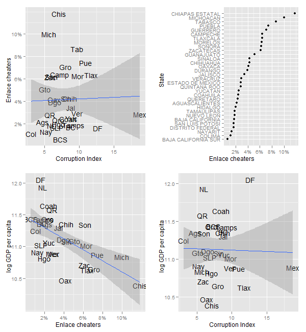
As for money being the root of all evil, there’s just not much evidence to support the Willie Sutton theory of Mexican Corruption. Cheating at school tests predicts corruption much better.

*A test of scholastic achievement taken by all sixth graders in Mexico

	########################################################
	##### Author: Diego Valle Jones
	##### Website: www.diegovalle.net
	##### Date Created: Thu Feb 18 19:34:27 2010
	########################################################
	#Corruption indicators and their correlations

	library(ggplot2)

	grid.newpage()
	pushViewport(viewport(layout = grid.layout(nrow = 2, ncol = 2)))

	subplot <- function(x, y) viewport(layout.pos.row = x,
	layout.pos.col = y)

	#The corruption data is from transparency international
	#The gdp from the INEGI
	#The percentage of cheaters from ENLACE
	cheats <- read.csv("http://spreadsheets.google.com/pub?key=tdkgy7KPm-mKN9rWa0ryIPA&single=true&gid=0&output=csv")
	print(ggplot(cheats2, aes(V1, log((gdp * 1000000) / pop),
	label = Abbrv)) +
	geom_text() +
	geom_smooth(method=lm) +
	scale_x_continuous(formatter = "percent") +
	ylab("log GDP per capita") +
	xlab("Enlace cheaters"),
	vp = subplot(2, 1))

	#exclude Campeche and Tabasco because they've got oil
	cheats2 <- cheats[-c(4,27),]
	print(ggplot(cheats2, aes(X2007, log((gdp * 1000000) / pop),
	label = Abbrv)) +
	geom_text() +
	geom_smooth(method = lm) +
	xlab("Corruption Index") +
	ylab("log GDP per capita"),
	vp = subplot(2, 2))
	summary(lm(I(log(gdp*1000000) / pop) ~ X2007, data = cheats2))

	print(ggplot(cheats, aes(X2007, V1,
	label = Abbrv)) +
	geom_text() +
	scale_y_continuous(formatter = "percent") +
	geom_smooth(method=lm) +
	xlab("Corruption Index") +
	ylab("Enlace cheaters"),
	vp = subplot(1, 1))


	cheats$State <- with(cheats, reorder(factor(State), V1))
	print(ggplot(cheats, aes(V1, State)) +
	geom_point() +
	scale_x_continuous(formatter = "percent") +
	xlab("Enlace cheaters"),
	vp = subplot(1, 2))

	dev.print(png, "cheats.png", width=600, height=650)

view raw cheaters.r hosted with ❤ by GitHub

Corruption indicators in Mexico

Newsletter and free shapefiles