Posted on Wed 14 July 2010

Homicide in North America


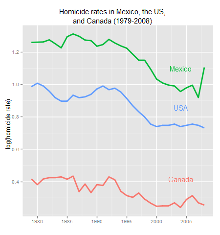
I’m surprised by how similar the trends are (excluding the drug war in Mexico). There were big decreases in the homicide rate in all three countries starting in the early nineties, which then slowed down around 2000.


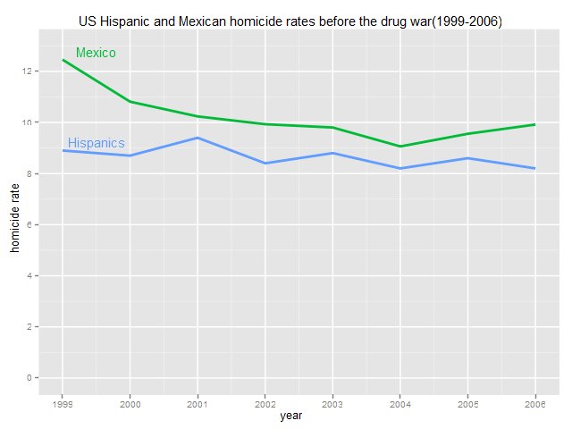
The homicide rates for Mexicans and Hispanics in the US are very similar, this is not surprising given that 2/3 of Hispanics are of Mexican descent (the median age in Mexico is 26 and among Hispanics 27). I wish there were data available for Hispanics before 1999 since there was a significant drop in the homicide rate in both Mexico and the US. If you look at the top chart the drop in the murder rate in the United States started slowing a couple of years before Mexico’s and that’s probably the reason for the bigger gap during the first years of the series.


Update: Here’s the first image with a log scale


########################################################
##### Author: Diego Valle Jones
##### Website: www.diegovalle.net
##### Date Created: Tue Jul 13 11:02:59 2010
########################################################
#1. -Compare homicide rates according Vital Statistics in the US (Hispanics) and in Mexico
#2.- Homicides in the three North American coutries
#Sources:
#INEGI Estadísticas Vitales for Mexico - http://github.com/diegovalle/Homicide-MX-Drug-War
#Centers for Disease Control and Prevention, National Center for Health Statistics. Compressed Mortality File 1999-2006. CDC WONDER On-line Database, compiled from Compressed Mortality File 1999-2006 Series 20 No. 2L, 2009. Accessed at http://wonder.cdc.gov/cmf-icd10.html on Jul 8, 2010 1:17:04 PM
library(ggplot2)
library(directlabels)
library(Cairo)
########################################################
#US Hispanics and Mexicans
#All Hispanics refers to Hispanics of all races
#Hispanics refers to White Hispanics. This is probably a better
#comparison since it excludes Black Hispanics (ie Puerto Ricans, etc)
#and we want to compare the rate with Mexico
########################################################
rates <- data.frame(year = c(1999:2006),
Mexico = c(12.45741755, 10.81080455, 10.23511614,
9.929701873, 9.801023152, 9.060029951,
9.555843656, 9.916635234),
#All.Hispanics = c(8.4, 8.3, 9, 8.1, 8.4, 7.9,
#8.2, 8),
Hispanics = c(8.9, 8.7, 9.4, 8.4, 8.8, 8.2, 8.6,
8.2))
mrates <- melt(rates, id = "year")
p <- ggplot(mrates, aes(year, value, group = variable,
color = variable)) +
geom_line(size=1) +
ylab("homicide rate") +
opts(title = "US Hispanic and Mexican homicide rates before the drug war(1999-2006)") +
scale_y_continuous(limits = c(0, 13)) +
scale_colour_manual(values = c("#00BA38", "#619CFF"))
get.pos <-
dl.indep(unique(transform(d,x = 1999.5, y = y[1]+.3)))
Cairo(file = "hispanics-vs-mexicans.png", width = 640, height = 480)
print(direct.label(p, "get.pos"))
dev.off()
########################################################
#Mexico, US and Canada
########################################################
#Mexico 1979-2008
#SINAIS - http://github.com/diegovalle/Homicide-MX-Drug-War
Mexico <- c(18.2359257110631, 18.2880765645248, 18.3428625694480,
18.9077374021619, 17.8847727425108, 16.8624511215753,
19.7674114887191, 20.5597966866621, 19.8879464890342,
18.8382270016049, 18.7001378513082, 17.2642907468046,
17.6775067520154, 19.0354212072118, 18.0773362506455,
17.34212109, 16.78286096, 15.40748018, 14.14614354,
14.14028699, 12.45741755, 10.81080455, 10.23511614,
9.929701873, 9.801023152, 9.060029951, 9.555843656,
9.916635234, 8.318309568, 12.77435165)
#Canda 1978-2008
#WTF Canada! you're not supposed to charge for statistics, not even
#a poor country like Mexico does that!
#http://ywcacanada.ca/data/research_docs/00000038.pdf
Canada <- c(2.76, 2.61, 2.41, 2.61, 2.66, 2.66, 2.69, 2.60, 2.72, 2.18,
2.43, 2.15, 2.41, 2.38, 2.69, 2.58, 2.19, 2.06, 2.01, 2.14,
1.96, 1.85, 1.77, 1.78, 1.78, 1.86, 1.74, 1.95, 2.06, 1.86,
1.80, 1.83)
#From 1950-2005
#Source: FBI, Uniform Crime Reports, 1950-2005
#http://bjs.ojp.usdoj.gov/content/homicide/tables/totalstab.cfm
#and for 2006-2008 from
#http://www.fbi.gov/ucr/cius2008/data/table_01.html
USA <- c(4.6, 4.4, 4.6, 4.5, 4.2, 4.1, 4.1, 4, 4.8,
4.9, 5.1, 4.8, 4.6, 4.6, 4.9, 5.1, 5.6, 6.2,
6.9, 7.3, 7.9, 8.6, 9, 9.4, 9.8, 9.6, 8.8,
8.8, 9, 9.7, 10.2, 9.8, 9.1, 8.3, 7.9, 7.9,
8.6, 8.3, 8.4, 8.7, 9.4, 9.8, 9.3, 9.5, 9,
8.2, 7.4, 6.8, 6.3, 5.7, 5.5, 5.6, 5.6, 5.7,
5.5, 5.6, 5.7, 5.6, 5.4 )
kyears <- 1979:2008
hom <- data.frame(year = kyears,
Canada = Canada[2:31],
Mexico = Mexico,
USA = USA[30:59]
)
mhom <- melt(hom, id = c("year"))
#International comparison
Cairo(file = "can-mx-us-homicide.png", width=450)
p <- ggplot(data = mhom, aes(year, value, group = variable,
color = variable)) +
geom_line(size = 1) +
labs(y = "homicide rate",x="") +
opts (title = "Homicide rates in Mexico, the US,\nand Canada (1979-2008)")
get.pos <-
dl.indep(unique(transform(d,x = 2004, y = y[length(x) - 4] + 1.5)))
print(direct.label(p, get.pos))
dev.off()


Unless otherwise stated, the content of this page is licensed under the Creative Commons Attribution 3.0 License, and code samples are licensed under the Apache 2.0 License. Privacy policy

Disclaimer: This website is not affiliated with any of the organizations or institutions to which Diego Valle-Jones belongs. All opinions are my own.

Special Projects:

Blogs I like: