library(mxmortalitydb)
library(stringr)
library(plyr)
library(ggplot2)
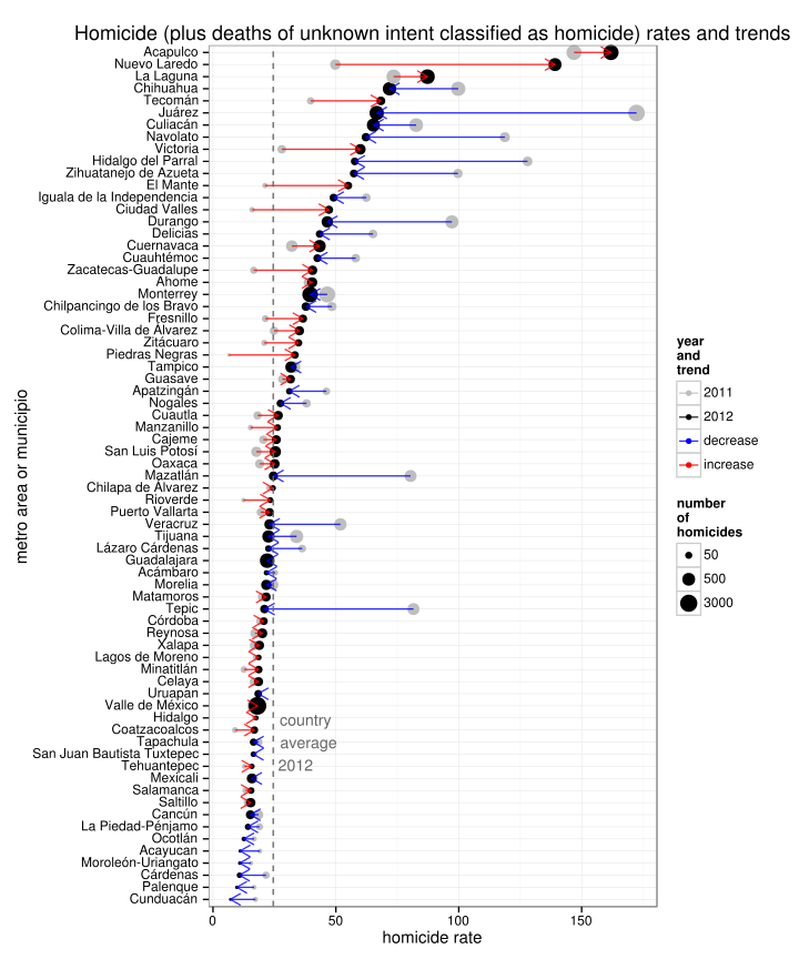
library(grid) ## needed for arrowplotMetro <- function(metro.name, metro.areas) { ## Plot the homicide counts in a metro area or municipio metro.name - name of ## the metro area to plot metro.areas - data frame containing a list of metro ## areas in the same format as the metro.area dataframe from mxmortalitydb ## data.frame metro.areas contains the 2010 CONAPO metro areas df <- merge(injury.intent, metro.areas, by.x = c("state_reg", "mun_reg"), by.y = c("state_code", "mun_code")) ## Yearly homicides in Mexico City, by state of registration df2 <- ddply(subset(df, metro_area == metro.name & intent.imputed == "Homicide"), .(year_reg), summarise, count = length(state_reg)) ggplot(df2, aes(year_reg, count)) + geom_line() + labs(title = str_c("Homicides (plus deaths of unknown intent classified as homicide) in\n", metro.name)) + ylim(0, max(df2$count)) + ylab("homicide count") + xlab("year of registration") + theme_bw() } plotChanges <- function(df, metro.areas, country.rate, years) { ## Plot of rates and trends df - injury.intent dataframr metro.areas - data ## frame containing a list of metro areas in the same format as the ## metro.area dataframe from mxmortalitydb country.rate - rate to show as a ## gray dotted line years - start and end year to compare changes ## Where the municipio where the death occurred is unknown use the municipio ## where it was registered as place of occurrancedf[df$mun_occur_death == 999, ]$mun_occur_death <- df[df$mun_occur_death == 999, ]$mun_reg ## Counts of homicide by state and municipio df <- ddply(subset(df, year_reg %in% years & intent.imputed == "Homicide"), .(state_occur_death, mun_occur_death, year_reg), summarise, count = length(state_reg)) ## Merge the counts with our fake metro areas df <- merge(df, metro.areas, by.x = c("state_occur_death", "mun_occur_death"), by.y = c("state_code", "mun_code")) ## Now get the counts by metro area (which may contain more than one ## municipio) df <- ddply(df, .(metro_area, year_reg), summarise, count = sum(count), population = sum(mun_population_2010), rate = count/population * 10^5) ## We are only interesed if the metro area at some time had a homicide rate ## of at least 15 df <- subset(df, metro_area %in% subset(df, rate > 15)$metro_area) ## Make sure the dataframe is ordered by metro and year df <- df[order(df$metro_area, df$year_reg), ] ## Order the chart by homicide rate in 2012 df$metro_area <- reorder(df$metro_area, df$rate, function(x) x[[2]]) ## Data frame for the arrow structure arrows <- ddply(df, .(metro_area), summarise, start = rate[1], end = rate[2], metro_area = metro_area[1], change = ifelse(rate[1] >= rate[2], "decrease", "increase")) ggplot(df, aes(rate, metro_area, group = as.factor(year_reg), color = as.factor(year_reg))) + geom_point(aes(size = log(count))) + labs(title = "Homicide (plus deaths of unknown intent classified as homicide) rates and trends") + scale_size("number\nof\nhomicides", breaks = c(log(50), log(500), log(3000)), labels = c(50, 500, 3000)) + geom_segment(data = arrows, aes(x = start, y = metro_area, xend = end, yend = metro_area, group = change, color = change), arrow = arrow(length = unit(0.3, "cm")), alpha = 0.8) + scale_color_manual("year\nand\ntrend", values = c("gray", "black", "blue", "red")) + ylab("metro area or municipio") + xlab("homicide rate") + # scale_x_log10()+ geom_vline(xintercept = country.rate, linetype = 2, color = "#666666") + annotate("text", y = "Tapachula", x = 25, label = "country\naverage\n2012", hjust = -0.1, size = 4, color = "#666666") + theme_bw() }
## Let's treat the big municipalities which are not part of a metro area as
## if they were one rename big.municipios to merge with metro.areas
big.municipios2 <- big.municipios
names(big.municipios2) <- c("state_code", "mun_code", "mun_population_2010",
    "metro_area")
metro.areas.fake <- rbind.fill(metro.areas, big.municipios2)
Changes from 2011 to 2012 and from the year before the drug war was declared to 2012:
plotChanges(injury.intent, metro.areas.fake, 24.5, c(2011, 2012))plotChanges(injury.intent, metro.areas.fake, 24.5, c(2006, 2012)) 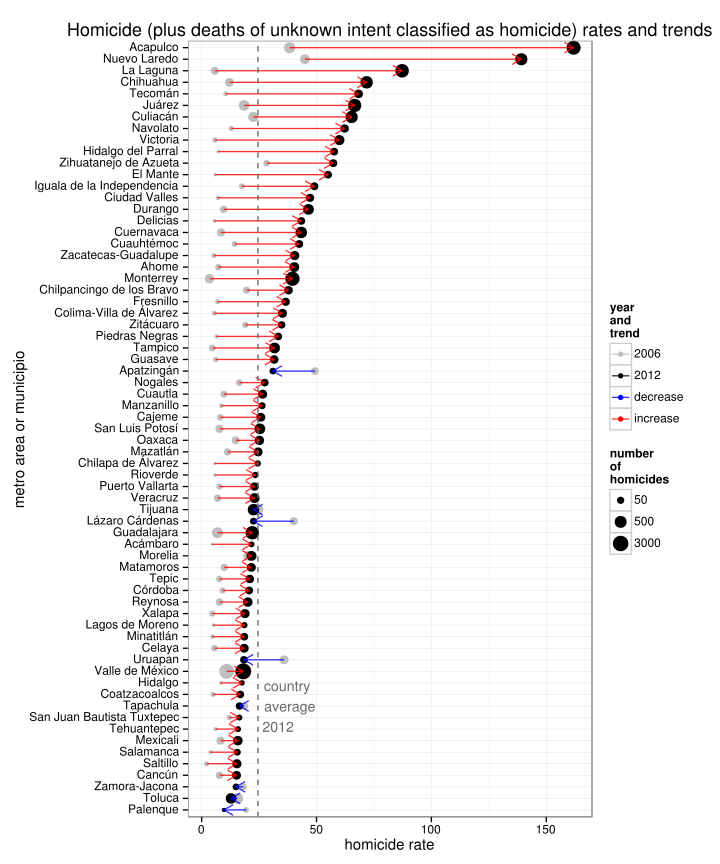
Do note that the charts were made using the 2010 population according to the CONAPO that comes with mxmortalitydb, so homicides in 2012 were overestimated by a little bit and underestimated by a little bit in 2006. Also rather than using the raw homicide numbers I adjusted them by classifying deaths of unknown intent.
ll <- list("Acapulco", "Nuevo Laredo", "La Laguna", "Chihuahua", "Tecomán",
"Juárez", "Culiacán", "Victoria", "Hidalgo del Parral", "Zihuatanejo de Azueta",
"El Mante", "Ciudad Valles", "Ciudad Valles", "Durango", "Cuernavaca", "Zacatecas-Guadalupe",
"Monterrey", "Piedras Negras", "Mazatlán", "Veracruz", "Tijuana", "Guadalajara",
"Tepic", "Coatzacoalcos")
names(ll) <- ll # make lapply print the names of the metro areas
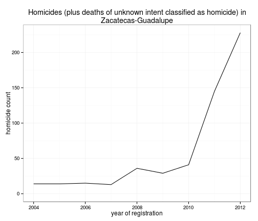
lapply(ll, plotMetro, metro.areas.fake)## $Acapulco
##
## $`Nuevo Laredo`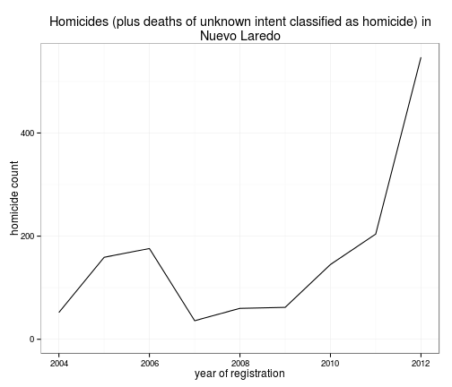
##
## $`La Laguna`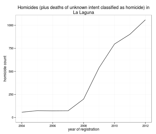
##
## $Chihuahua
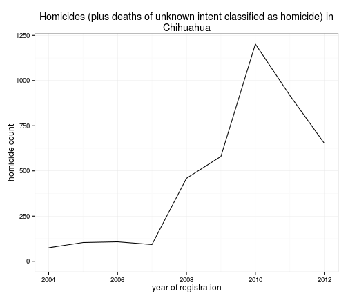
##
## $Tecomán
##
## $Juárez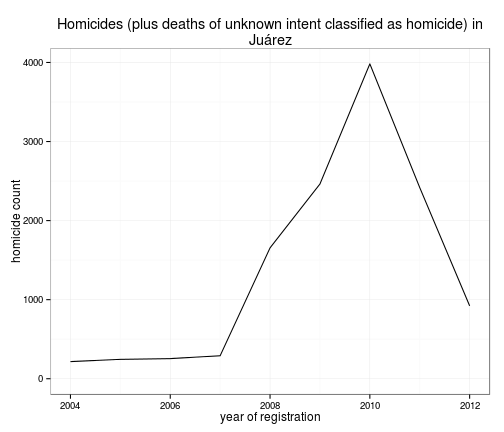
##
## $Culiacán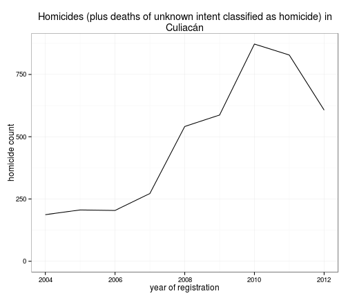
##
## $Victoria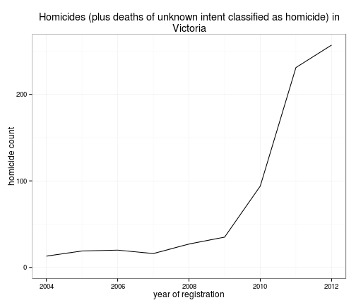
##
## $`Hidalgo del Parral`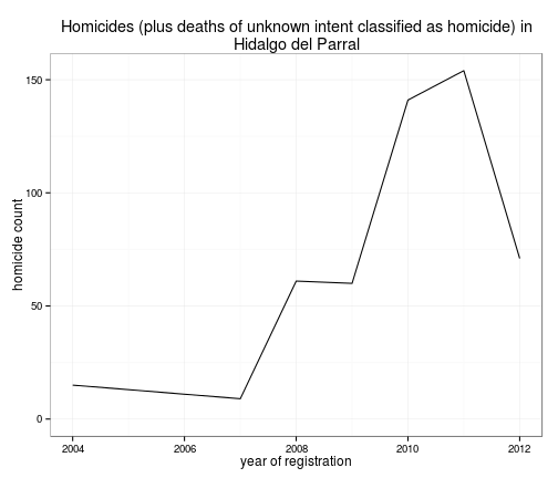
##
## $`Zihuatanejo de Azueta`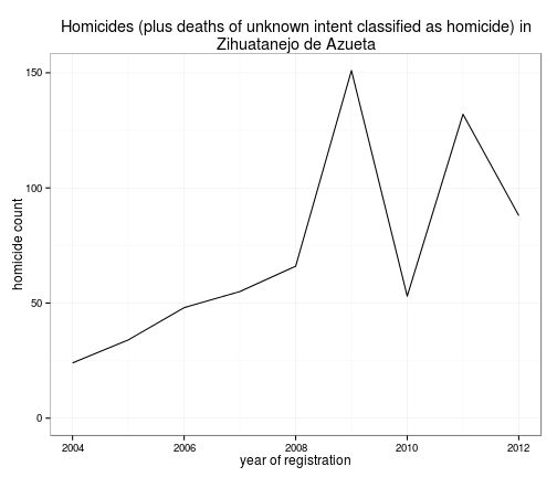
##
## $`El Mante`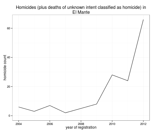
##
## $`Ciudad Valles`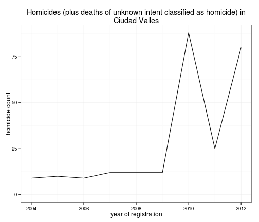
##
## $Durango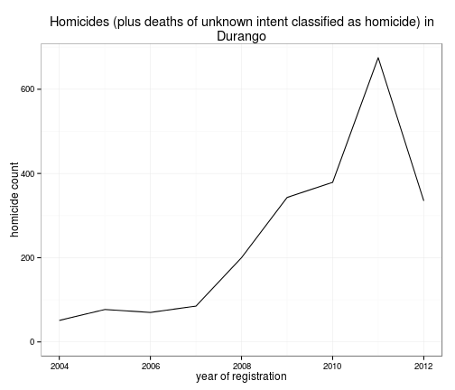
##
## $Cuernavaca
##
## $`Zacatecas-Guadalupe`
##
## $Monterrey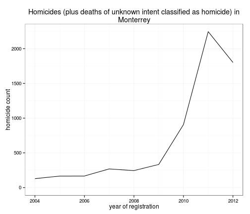
##
## $`Piedras Negras`
##
## $Mazatlán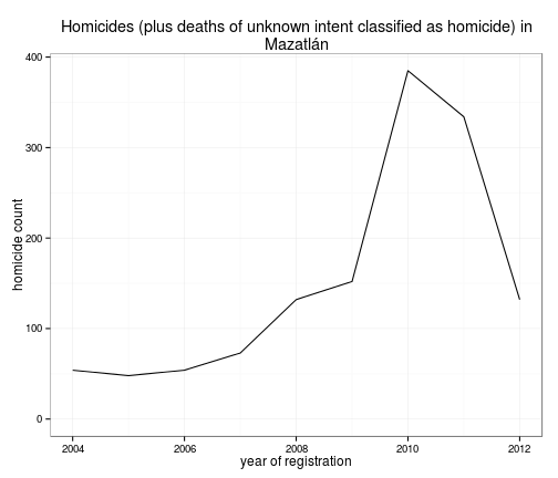
##
## $Veracruz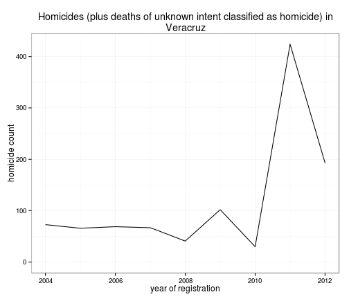
##
## $Tijuana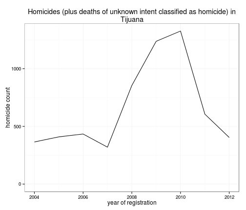
##
## $Guadalajara
##
## $Tepic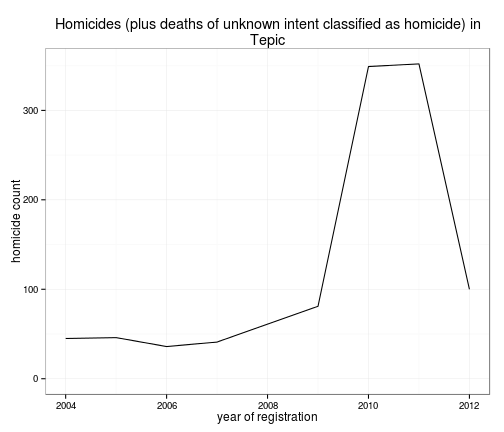
##
## $Coatzacoalcos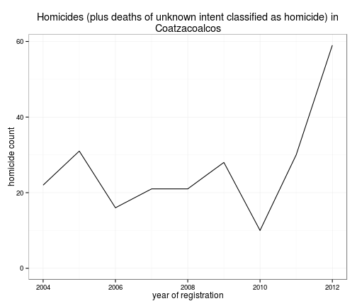
Check out the source code as an R markdown file.